ABSTRACT

I use extreme value theory and estimate a Generalized Pareto distribution for wholesale electricity prices using data from seven trading hubs in the United States. My estimates of the shape parameter indicate that the distribution of wholesale electricity prices is fat-tailed. I also explore whether the shape parameter for this distribution changes during the summer months, which are the peak months for electricity usage in the United States. My estimates suggest that for most trading hubs the shape parameter does not vary during the summer months. I also present return levels for prices, which can be viewed as the waiting time for worst-case scenarios for prices, and compare realizations of prices with them.

Keywords and Phrases: Extreme Value Theory; Generalized Pareto Distribution; Fat-tails; Electricity Prices; Return Levels.

1. INTRODUCTION

Tail risk is a term that is being used more commonly these days, with references in areas as diverse as financial markets, environmental and climatic disasters as well as public health.^[1] These tail risks represent low probability events that are in the tails of a distribution. However, even though these events have a low probability of occurring they can have outsized effects and serious consequences when they do occur, e.g., large financial losses, devastating storm damage or huge mortality during a pandemic.

In financial and commodity markets these tail risks can manifest as price spikes, which represent sudden price swings. In electricity markets, storage is difficult, which means that it can be difficult to balance the market for electricity at different parts of the cycle. For example, the demand for electricity can exceed generating capacity and as there is so little electricity in storage to act as a buffer, this can lead to large price swings. Consequently, modelling the probability of these sorts of price swings is important from a risk management perspective.

Extreme value theory is one tool that can be used to assess the probability of these extreme price movements or tail risks. As noted by Cirillo and Taleb, extreme value theory emphasizes that the tails of the distribution contain more information than the values that are observed more frequently.^[2] Consequently, extreme value theory is a viable tool for managing the risks associated with these extreme price swings. Moreover, extreme value theory can be useful even in cases with a small number of observations.^[3] This has certainly been recognized in the banking industry for risk management.^[4]

I study wholesale electricity prices from several trading hubs in the United States. I apply extreme value theory to these data and estimate the distribution of wholesale electricity prices. While some earlier work using extreme value theory has considered European and Canadian electricity markets,^[5] the electricity prices from the United States have not been studied using this perspective. My approach focuses on price data that exceeds a threshold to estimate a Generalized Pareto distribution with a maximum likelihood estimator.^[6] Maximum likelihood proceeds by assuming a distribution for the data and creating a likelihood function that provides a complete probabilistic description of the data and then picking the parameters of the distribution to maximize the likelihood function.

In order to examine whether there is a good chance of an extreme event, in this case, wholesale electricity prices, I will consider the estimate of the “shape parameter” of the distribution of prices. The shape parameter of the distribution is quite informative as it indicates how fat the tails of the distribution are. “Fat tails” is a statistical term indicating how likely outliers, e.g., extreme events, are to occur. With a normal distribution, a thin tailed distribution, extreme events are quite rare and have a low probability of occurring. Generally speaking, extreme prices are more common in a distribution with fatter tails.

My estimates of the shape parameter are all consistent with a fat-tailed Pareto distribution.^[7] Moreover, I can rule out alternative distributions that have thinner tails such as the Beta and exponential distributions.^[8] I use the estimates of the distribution from each of the hubs I consider to compute the return levels, which present the likelihood that an “extreme” value is observed in the future. These return levels can be viewed as the time before observing an extreme price event for the wholesale prices to return to normal. As such, return levels are also known as the waiting time for worst-case scenarios for wholesale electricity prices in each of the trading hubs that I consider. The return levels are thus a way to quantify the tail risks in electricity prices.

Finally, I also consider how the distribution of electricity prices could differ across seasons (i.e., summer months, which are the peak months for electricity consumption in the United States, versus the other months of the year), by estimating a specification that makes the shape parameter a function of this seasonal dummy.

In the next section of the paper, I discuss the data used and provide some background on extreme value theory as well as my estimation approach. The empirical results are presented and discussed in Section 3. I present a summary of my estimates and their implications in Section 4.

2. DATA AND EMPIRICAL METHODS

The wholesale electricity price data used were obtained from the U.S. Energy Information Administration (EIA).^[9] I focus on the daily high price for electricity contracts (price per megawatt hour (MWh)) traded for seven major trading hubs (over the counter markets) in the United States. Electricity trading on these hubs reflects purchases and sales by power stations, utilities, chemical and transportation companies, financial institutions, hedge funds, as well as other energy market participants. The trading hubs, as well as their respective regions, considered are: the MASS hub (the New England region); the PJM hub (Pennsylvania, New Jersey, Maryland, Ohio and parts of Tennessee); the INDIANA hub (Midwestern states); the MID-COLUMBIA hub (states in the Pacific Northwest); the PALO VERDE hub (the southwestern states); the NP15 hub (Northern California); and, the SP15 hub (Southern California).^[10] The availability of the data varies by hub, with some hubs having data as far back as 2001 (e.g., MASS and PJM) and others beginning later (e.g., 2006 for the INDIANA and 2009 for NP15 hubs).

I present some descriptive statistics for the price data in Table 1. As can be seen in Table 1 the mean price is greater than the median price, which suggests that the distribution of maximum daily prices is skewed to the right in all the hubs I consider. The skewness coefficients indicate that the skewness in the price data varies a great deal across hubs. There is also a great deal of dispersion in the electricity price data, as indicated by the standard deviation of the price, and this also varies a great deal by hub. Finally, the kurtosis measures for the price data are quite large. Recall that a normal distribution has a kurtosis measure of 3, which suggests that the price data from these trading hubs have quite thick tails and therefore may be prone to extreme, low probability events.

Let x₁, …, x_N be independently and randomly distributed random variables from an unknown distribution function F(x). As shown in Coles,^[11] and elsewhere, the distribution of the values of x that exceed a threshold u is defined by

If the threshold level F_u(ϵ) is sufficiently large then the distribution can be approximated by a Generalized Pareto distribution, which has cumulative distribution function

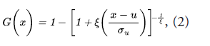
where u is a threshold, x > u, σ_u is a scale parameter, which depends on the threshold u and determines the dispersion or spread in the distribution, and is such that σ_u > 0 and ξ is a shape parameter. In addition, the Generalized Pareto distribution has an infinite mean if ξ > 1 and infinite variance if ξ > 1/2. The shape parameter, ξ, is also key for determining the nature of the tails of the distribution. In particular, when ξ > 0 the distribution is fat-tailed (i.e., a Pareto). In contrast, the thinner tailed Beta and exponential distribution result when ξ < 0 and ξ → 0, respectively. I obtain my estimates using a maximum likelihood estimator.

The estimates of the parameters of the Generalized Pareto distribution can also be used to compute the return level x_m, i.e., a level that is exceeded once every m^th year,

where m is large enough so that x_m > u and the notation is as defined earlier. The return levels provide some indication of the likelihood of spikes in the price of electricity that exceed the threshold level in the future. The return levels are thus useful and important from a risk management perspective, as they provide an indication of the sorts of price spikes in wholesale electricity prices we could observe in the future.

I also explored whether the shape parameter might vary by season. In particular, I estimated a model that makes the shape parameter a function of an intercept and an indicator variable that takes the value 1 for a summer month (which I defined as June, July and August) and 0 otherwise. This alternative specification means that the shape parameter of the distribution for electricity will vary by season instead of being constant across all seasons. In the United States, the summer tends to be the peak season for electricity usage. Consequently, this specification sheds light on whether the distribution varies by the peak season. For example, do distributions of electricity prices have heavier tails during the summer months or is the distribution constant across seasons? If the coefficient estimate on the indicator for a summer month is not statistically different from zero, this suggests that the shape parameter of the distribution for electricity prices does not vary across seasons.

The value of the threshold in equations (1) and (2) is not known and must be determined based on the data. As with most things in statistics, there is a bit of a trade-off when selecting the threshold. One needs to pick a threshold that is large enough to satisfy the theory underlying equation (1), but doing so can result in small samples that can create imprecise estimates and suffer from small sample biases. There are a few approaches for selecting the value of the threshold. On the one hand, “the eyeball method” where one examines plots of the residuals (mean residual life plot)^[12] to determine where the plot exhibits linearity, with the threshold being the point at which linearity appears in the plot. On the other hand, the Hill approach where the threshold is estimated using the Hill estimator.^[13] I focus on using the Hill estimator to select the threshold, but my selections for the threshold using the eyeball method tend to be similar to those picked by the Hill estimator for most of the hubs I consider. I present these threshold values in Table 2. Table 2 also presents the number of observations that exceed the threshold value selected by the Hill estimator. As can be seen in Table 2, the number of observations above the thresholds selected by the Hill estimator tends to vary across hubs with the largest samples of observations above the thresholds in the MASS (Massachusetts), Mid-Columbia and Palo Verde hubs.

I obtain my maximum likelihood estimates of the Generalized Pareto distribution using the R package extRemes.^[14]

3. EMPIRICAL RESULTS

I present estimates of the scale and shape parameters of the Generalized Pareto distribution for wholesale electricity price for each trading hub and use these estimates to compute the return levels. I divide my data on prices into a training and a test sample, where the test sample contains the last year of data available for each of the trading hubs. I fit the models with the training data and use these estimates to compute the return levels. I compare the return levels with the test data to assess how frequently realizations of prices appear in the confidence intervals of the return levels.

The estimates of the parameters of the Generalized Pareto distribution by trading hub are presented in Table 3. The estimates in Table 3 show that the shape parameter estimates for each of the trading hubs are all positive and have confidence intervals that do not cross zero. This indicates that the distributions of electricity prices are all consistent with the Pareto distribution. In addition, I can also rule out thinner tailed alternatives like the exponential and Beta distributions. The shape parameter estimates indicate that the distribution for electricity prices would have finite mean and variance in all but one of the hubs I consider. The shape parameter estimate for the SP15 hub is greater than 0.5, which indicates that the variance for the distribution of electricity prices from this hub is infinite. An infinite variance suggests that extreme price movements are much more likely to be observed.

The return levels for each of the hubs, which are based on the estimates in Table 3 for the training data, are presented in Figure 1 with 95 per cent confidence intervals. As discussed earlier, I also took the last year of data available and saved it as “test” data, and determined how the maximum price in the test data compares with the return levels computed using the training data. This is a validation exercise where I examine how well the return levels coincide with extreme prices out-of-sample. In the Mid-Columbia and Palo Verde hubs the maximum price in the test data exceeded all the return levels plotted in Figure 1 for these hubs. The maximum high price during the test period for the MASS, NP15 and SP15 hubs ($290, $367.95 and $395/MWh) are all contained within the confidence intervals at various horizons presented for the return levels. For the remaining hubs (Indiana and Mid-Columbia), the maximum price during the test period is not contained in the confidence intervals for any of the return levels plotted in Figure 1. This suggests that the out-of-sample validation in some of the hubs is not as strong as in some of the others.

Finally, I present the estimates of the Generalized Pareto distribution where the shape parameter is specified as a function of an intercept and an indicator for the summer months. These estimates are presented in Table 4. Overall, most of the estimates in Table 4 indicate that the summer dummy does not have statistically significant estimates, which suggests that the distribution of electricity prices does not vary across seasons for the trading hubs. However, I did find statistically significant estimates on the summer dummy in two hubs. First, the summer dummy has a negative estimate that is statistically significant at the 5 percent level of significance for the Massachusetts hub.^[15] While the estimate is negative, the estimates of the slope and intercept for the Massachusetts hub indicate that the distribution of electricity prices would still be a fat-tailed Pareto distribution, although the shape parameter would be smaller during the summer. Second, the Palo Verde hub, which covers the hot and arid U.S. southwest, has a positive estimate on the summer dummy that is statistically significant at the 10 per cent level of significance. This suggests that the distribution of electricity prices in this hub has a bigger shape parameter during the summer months. As discussed earlier, the shape parameter presented in Table 3 for the Palo Verde hub exceeds 0.5, so the distribution of electricity prices during the summer months is still consistent with a distribution with infinite variance.

The relative homogeneity of the distribution for electricity prices in most of the trading hubs is noteworthy, as the demand for electricity tends to be greatest during the summer in the United States. While the demand for electricity does peak during the summer, this seasonal change does not affect the tails of the distribution for electricity prices in most of the trading hubs. This differs somewhat from the findings in Walls and Zhang for electricity prices in the Canadian province of Alberta.^[16] Walls and Zhang divided their data into summer and winter months and estimated generalized Pareto distributions for these two periods.^[17] While the distribution for both the summer and winter months are fat-tailed, the estimated shape parameter of the distribution during the summer months differs a great deal from the estimates for the winter months. While I use U.S. data in my analysis there are some implications for Canada. The energy-wholesale market in Alberta may increase the possibility of extreme price events if demand spikes during peak periods. Consequently, one would expect larger estimates of the shape parameter for the Generalized Pareto distribution. For example, Walls and Zhang do obtain larger shape parameter estimates for Alberta than those I present, which is consistent with a distribution of wholesale electricity prices that may be more prone to extreme price movements.^[18] In other provinces, without organized wholesale markets, the implications are more difficult to ascertain via price movements, but the consequences of spikes in demand will manifest via other means.

4. DISCUSSION AND CONCLUDING REMARKS

I apply extreme value theory to wholesale electricity prices from several trading hubs in the United States. I use electricity prices that exceed a threshold to estimate a Generalized Pareto distribution with maximum likelihood. I find that the distribution is fat-tailed and I can rule out thinner tailed alternatives, such as the exponential and Beta distributions. Moreover, I also find that the shape parameter of the distribution does not vary during the summer months in most of the trading hubs, which suggests that the thickness of the tails of the distribution of wholesale electricity prices is not likely to change during the summer months of peak electricity usage. This is a somewhat surprising result as demand for electricity tends to increase during the summer. If the shape parameter did become larger during the summer months, that would suggest that the distribution would be fatter-tailed during the summer and extreme price movements are more likely relative to the other seasons. Finally, I also present the return levels for electricity prices in each of these hubs. Not surprisingly, the return levels vary considerably across hubs, which suggests that risk management for price surges should be based on data for a particular hub.

Table 1: Descriptive Statistics for Daily High Price of Electricity (MWh)^[19]

Notes: price reported is for megawatt hour (MWh) for maximum daily price. Total number of observations is for all observations during the sample period listed.

Table 2: Threshold Values

Notes: Threshold value is price per megawatt hour (MWh); Number of observations above the threshold selected by the Hill estimator is presented above. To implement the eyeball method, I examine the mean residual life plot and pick the threshold level to be the point (vicinity) where the plot begins to exhibit linearity.

Table 3: Estimates of the Generalized Pareto Distribution for Wholesale Electricity Price by Trading Hub, using the training data

Notes: Standard errors in parentheses. *** denotes statistical significance at the 1 percent level; ** denotes statistical significance at the 5 percent level. The estimates are based on the training data, which excludes the last year of data I have available, and are indicated in parentheses in the first column of the table.

Table 4: Estimates of the Generalized Pareto Distribution for Wholesale Electricity Price by Trading Hub, shape parameter a function of a summer dummy, using the training data

Notes: Standard errors in parentheses. *** denotes statistical significance at the 1 percent level; ** denotes statistical significance at the 5 percent level; * denotes statistical significance at the 10 percent level. The estimates are based on the training data, which excludes the last year of data I have available, and are indicated in parentheses in the first column of the table.

Figure 1: Return Level Plots by Trading Hub for Wholesale Electricity Price

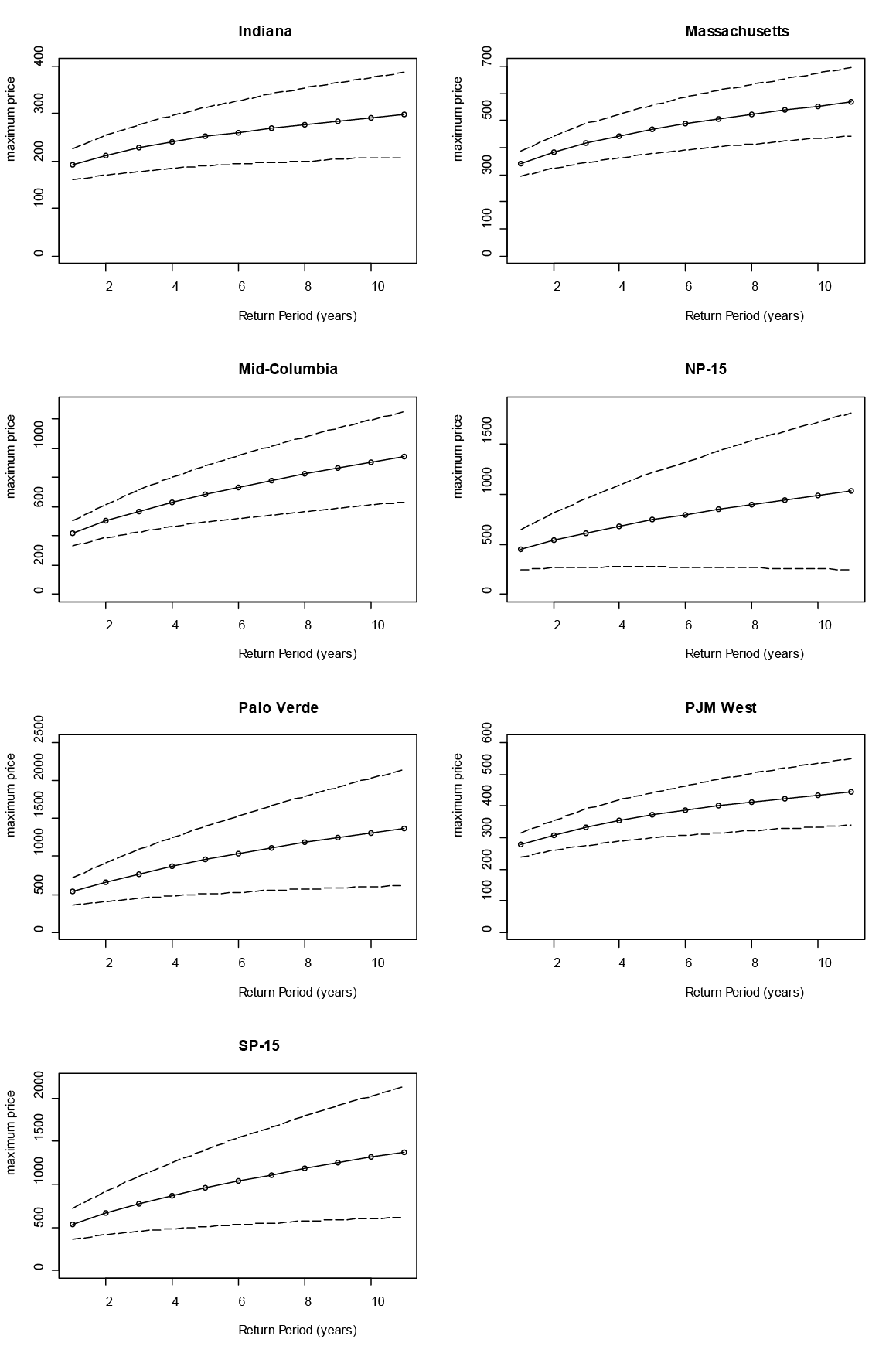
Notes: Dashed line denotes 95 percent confidence bounds.

• * Michele Campolieti is Professor of Economics at the Department of Management, University of Toronto Scarborough. The data and R scripts used in this paper are available upon request. This research did not receive any specific grant/financial support from funding agencies in the public, commercial, or not-for-profit sectors. Please address correspondence to: Michele Campolieti, Department of Management, University of Toronto Scarborough, 1095 Military Trail, Toronto, Ontario, M1C 1A4; Voice: 416-978-2748; email: campolie@chass.utoronto.ca.

  ¹ Nassim Nicholas Taleb, Statistical Consequences of Fat Tails: Real World Preasymptotics, Epistemology, and Applications (STEM Academic Press, 2020); Saralees Nadarajah, “Extremes of Daily Rainfall in West Central Florida”(2005) 69 Climatic Change 325; VF Pisarenko & Didier Sornette, “Characterization of the Frequency of Extreme Earthquake Events by the Generalized Pareto Distribution” (2003) 160 Pure & Applied Geophysics 2343; Pasquale Cirillo & Nassim Nicholas Taleb, “Tail Risk of Contagious Diseases” (2020) 16 Nature Physics 606; Michele Campolieti, “Tail Risks and Infectious Disease: Influenza Mortality in the U.S., 1900–2018” (2021) 6 Infectious Disease Modelling 1135.

• ² Cirillo & Taleb, supra note 1.

• ³ Ibid.

• ⁴ Basel Committee on Banking Supervision, Enhancements to the Basel II framework (Basel: Bank for International Settlements, 2009).

• ⁵ WD Walls & Wei Zhang, “Using Extreme Value Theory to Model Electricity Price Risk with an Application to the Alberta Power Market” (2005) 23:5 Energy Exploration & Exploitation 375; Hans NE Byström, “Extreme Value Theory and Extremely Large Electricity Price Changes” (2005) 14:1 Intl Rev Econs & Finance 41; Kam Fong Chan & Philip Gray, «Using Extreme Value Theory to Measure Value-at-Risk for Daily Electricity Spot Prices» (2006) 22:2 Intl J Forecasting 283; F Paraschiv, R Hadzi-Mishev & D Keles, “Extreme Value Theory for Heavy Tails in Electricity Prices” (2016) 9 J Energy Markets 21; Efthymios Stathakis, Theophilos Papadimitriou & Periklis Gogas, “Forecasting Price Spikes in Electricity Markets” (2021) 13:1 Rev Econ Analysis 65.

• ⁶ Stuart Coles, An Introduction to Statistical Modeling of Extreme Values (London, UK: Springer-Verlag, 2001); Samuel Kotz & Saralees Nadarajah, Extreme Value Distributions: Theory and Applications (London, UK: Imperial College Press, 2000).

• ⁷ Pareto (power law) distributions are continuous distributions known for being skewed and concentrated. For example, Pareto’s rule where 20 percent of households own 80 per cent of wealth can be described by a Pareto distribution. There are many applications of Pareto distributions (capturing this sort of concentration) in economics, finance and science.

• ⁸ Beta distributions are continuous distributions for data that takes values between 0 and 1 and are often used to describe the distributions of percentages and proportions. An exponential distribution is for positive variables and is sometimes used in statistics and engineering to model waiting times.

• ⁹ The data are available from the U.S. Energy Information Administration (EIA) and are provided to the EIA by the Intercontinental Exchange (ICE). See US Energy Information Administration, “Wholesale Electricity and Natural Gas Market Data” (last modified 28 August 2026), online: <eia.gov/electricity/wholesale>.

• ¹⁰ I exclude data from the ERCOT hub, which covers Texas, as the data have not been updated since 2019 (the last year of data recorded in this hub).

• ¹¹ Coles, supra note 6.

• ¹² Coles, supra note 6; Eric Gilleland & Richard W Katz, «extRemes 2.0: An Extreme Value Analysis Package in R” (2016) 72:8 J Statistical Software 1, DOI: <10.18637/jss.v072.i08>.

• ¹³ The Hill estimator can be computed as , where X_i,n is the i-th order statistic of X₁, …, X_n, k(n)ϵ{1, …, n–1}.

• ¹⁴ Gilleland & Katz, supra note 12.

• ¹⁵ The Massachusetts differs from the other U.S. hubs in that peak use is in the winter months. This is consistent with the negative estimate on the indicator for summer months I obtain.

• ¹⁶ Walls & Zhang, supra note 5.

• ¹⁷ Ibid. Walls and Zhang defined the winter months as October to May and the summer months as June to September.

• ¹⁸ Ibid.

• ¹⁹ Descriptive Statistics for Daily High Price of Electricity (MWh), by Trading Hub. Author’s calculations based on US Energy Information Administration, supra note 9.